Just as the term Artificial Intelligence (AI) has been despised for many years, right in 2017 ‘Big Data’ begins something that generates more rejection than acceptance due to daily wear and bombing. Everything is Big Data and everything is solved with Big Data. But then, what do we do those whom work on Big Data?
Big Data has been related in recent years to large amounts of structured or unstructured data produced by systems or organizations. Its importance lies not in the data itself, but in what we can do with that data. On how data can be analyzed to make better decisions. Frequently, much of the value that can be extracted from data comes from our ability to process them in time. Hence, it is important to know very well both the data sources and the framework in which we are going to process them.
One of the initial objectives in all Big Data projects is to define the processing architecture that best adapts to a specific problem. This includes an immensity of possibilities and alternatives:
- What are the sources?
- How is the data stored?
- Are there any computational constraints? And of time?
- What algorithms should we apply?
- What accuracy should we reach?
- How critical the process is?
We need to know our domain very well in order to be able to answer these questions and provide quality answers. Throughout this post, we will propose a simplification of a real use case and compare two Big Data processing technologies.
Use case
The proposed use case is the application of the Kappa architecture for processing Netflow traces, using different processing engines.
Netflow is a network protocol to collect information about IP traffic. It provides us with information such as the start and end dates of connections, source and destination IP addresses, ports, protocols, packet bytes, etc. It is currently a standard for monitoring network traffic and is supported by different hardware and software platforms.
Each event contained in the netflow traces gives us extended information of a connection established in the monitored network. These events are ingested through Apache Kafka to be analyzed by the processing engine -in this case Apache Spark or Apache Flink-, performing a simple operation such as the calculation of the Euclidean distance between pairs of events. This type of calculations are basic in anomaly detection algorithms.
However, in order to carry out this processing it is necessary to group the events, for example through temporary windows, since in a purely streaming context the data lack a beginning or an end.
Once the netflow events are grouped, the calculation of distances between pairs produces a combinatorial explosion. For example, in case we receive 1000 events / s from the same IP, and we group them every 5s, each window will require a total of 12,497,500 calculations. The strategy to be applied is totally dependent on the processing engine. In the case of Spark, event grouping is straightforward as it does not work in streaming but instead uses micro-batching, so the processing window will always be defined. In the case of Flink, however, this parameter is not mandatory since it is a purely streaming engine, so it is necessary to define the desired processing window in the code.
The calculation will return as a result a new data stream that is published in another Kafka topic, as shown in the following figure. In this way a great flexibility in the design is achieved, being able to combine this processing with others in more complex data pipelines.

Kappa Architecture
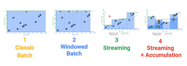
The Kappa architecture is a software architecture pattern that uses data streams or “streams” instead of using data already stored and persisted. The data sources will be, therefore, immutable and continuous, such as the entries generated in a log. These sources of information contrast with the traditional databases used in batch or batch analysis systems.
These “streams” are sent through a processing system and stored in auxiliary systems for the service layer.
The Kappa architecture is a simplification of the Lambda architecture, from which it differs in the following aspects:
- Everything is a stream (batch is a particular case)
- Data sources are immutable (raw data persists)
- There is a single analytical framework (beneficial for maintenance)
- Replay functionality, that is, reprocessing all the data analyzed so far (for example, when having a new algorithm)
In summary, the batch part is eliminated, favoring an in motion data processing system.
Get our hands dirty
To better understand all these theoretical concepts, nothing better than to deepen the implementation. One of the elements we want to put into practice with this proof of concept is to be able to exchange among different processing engines in a transparent way. In other words, how easy is switching between Spark and Flink based on the same Scala code? Unfortunately, things are not so straightforward, although it is possible to reach a common partial solution, as you can see in the following sections.
Netflow events
Each Netflow event provides information about a specific connection established in the network. These events are represented in JSON format and are ingested in Kafka. For simplicity, only IPv4 connections will be used. Example of event:
{ “eventid”:995491697672682, “dvc_version”:“3.2”, “aproto”:“failed”, “src_ip4”:168099844, “dst_ip4”:4294967295, “eventtime”:1490024708, “out_packets”:1, “type”:“flow”, “dvc_time”:1490024739, “dst_ip”:“255.255.255.255”, “src_ip”:“10.5.0.4”, “duration”:0, “in_bytes”:0, “conn_state”:“new”, “@version”:“1”, “out_bytes”:157, “dvc_type”:“suricata”, “in_packets”:0, “nproto”:“UDP”, “src_port”:42126, “@timestamp”:“2017-03-20T15:45:08.000Z”, “dst_port”:40237, “category”:“informational” }
Shared part
As mentioned above, one of the objectives of this article is to transparently use different Big Data processing environments , that is, to use the same Scala functions for Spark, Flink or future frameworks. Unfortunately, the peculiarities of each framework have meant that only a part of the Scala code implemented can be common for both.
The common code includes the mechanisms to serialize and deserialize netflow events. We rely on the json4s library of Scala, and define a case class with the fields of interest:
case class Flow_ip4(eventid: String, dst_ip4: String, dst_port: String, duration: String, in_bytes: String, in_packets: String, out_bytes: String, out_packets: String, src_ip4: String, src_port: String) extends Serializable
In addition, the Flow object that implements this serialization is defined to be able to work comfortably with different Big Data engines:
class Flow(trace: String) extends Serializable { implicit val formats =DefaultFormats var flow_case : Flow_ip4 = parse(trace).extract[Flow_ip4] def getFlow() : Flow_ip4 = flow_case }
Another code shared by both frameworks are the functions to calculate the Euclidean distance, obtain the combinations of a series of objects and to generate the Json of results:
object utils { def euclideanDistance(xs: List[Double], ys: List[Double]) = { sqrt((xs zip ys).map { case (x,y)=> pow(y – x, 2) }.sum) } def getCombinations(lists : Iterable[Flow_ip4]) = { lists.toList.combinations(2).map(x=> (x(0),x(1))).toList } def getAllValuesFromString(flow_case : Flow_ip4) = flow_case.productIterator.drop(1) .map(_.asInstanceOf[String].toDouble).toList def calculateDistances(input: Iterable[Flow_ip4]): List[(String, String, Double)] = { val combinations: List[(Flow_ip4, Flow_ip4)] = getCombinations(input) val distances = combinations.map{ case(f1,f2) => (f1.eventid,f2.eventid,euclideanDistance(getAllValuesFromString(f1), getAllValuesFromString(f2)))} distances.sortBy(_._3) } def generateJson(x: (String, String, Double)): String = { val obj = Map(“eventid_1” -> x._1, “eventid_2” -> x._2, “distance” -> x._3, “timestamp” -> System.currentTimeMillis()) val str_obj = scala.util.parsing.json.JSONObject(obj).toString() str_obj } }
Specific part of each Framework
The application of transformations and actions is where the particularities of each framework prevent it from being a generic code. As observed, Flink iterates by each event, filtering, serializing, grouping by IP and time and finally applying distance calculation to send it out to Kafka through a producer. In Spark, on the other hand, since events are already grouped by time, we only need to filter, serialize and group by IP. Once this is done, the distance calculation functions are applied and the result can be sent out to Kafka with the proper libraries.
| Flink |
val flow = stream .filter(!_.contains(“src_ip6”)) .map(trace =>{ new Flow(trace).getFlow() }) .keyBy(_.src_ip4) .timeWindow(Time.seconds(3)) .apply{( key: String, window: TimeWindow, input: Iterable[Flow_ip4], out: Collector[List[(String,String, Double)]]) => { val distances: List[(String, String, Double)] = utils.calculateDistances(input) out.collect(distances) } } .flatMap(x => x) flow.map( x=>{ val str_obj: String = utils.generateJson(x) producer.send(new ProducerRecord[String, String](topic_out, str_obj)) }) |
| Spark |
| val flow = stream.map(_.value()) .filter(!_.contains(“src_ip6”)) .map(record => { implicit val formats = DefaultFormats val flow = new Flow(record).getFlow() (flow.src_ip4,flow) }) .groupByKey() flow.foreachRDD(rdd => { rdd.foreach{ case (key, input ) => { val distances = utils.calculateDistances(input) distances.map(x => { val str_obj: String = utils.generateJson(x) producer.send(new ProducerRecord[String, String](topic_out, str_obj)) }) }} }) |
The IDs of each event, their ingestion timestamps, the result of the distance calculation and the time at which the calculation was completed are stored in the Kafka output topic. Here is an example of a trace:
{ “eventid_1”:151852746453199<spanstyle=’font-size:9.0pt;font-family:”Courier New”;color:teal’>, “ts_flow1”:1495466510792, “eventid_2”:1039884491535740, “ts_flow2”:1495466511125, “distance”:12322.94295207115, “ts_output”:1495466520212 }
Results
We have run two different types of tests: multiple events within a single window, and multiple events in different windows, where a phenomenon makes the combinatorial algorithm apparently stochastic and offers different results. This occurs due to the fact that data is ingested in an unordered manner, as they arrive to the system, without taking into account the event time, and groupings are made based on it, which will cause different combinations to exist.
The following presentation from Apache Beam explains in more detail the difference between processing time and event time: https://goo.gl/h5D1yR
Multiple events in the same window
About 10,000 events are ingested in the same window, which, applying the combinations for the same IPs, require almost 2 million calculations. The total computation time in each framework (i.e. the difference between the highest and the lowest output timestamp) with 8 processing cores is:
- Spark total time: 41.50s
- Total time Flink: 40,24s
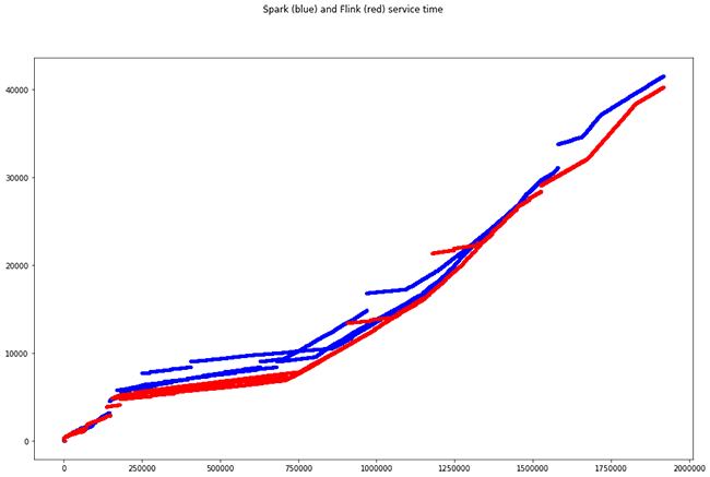
Las múltiples líneas de un mismo color se deben al paralelismo, existiendo cálculos que terminan en el mismo momento temporal
Multiple events in different windows
More than 50,000 events are inserted along different time windows of 3s. This is where the particularities of each engine clearly arise. When we plot the same graph of processing times, the following occurs:
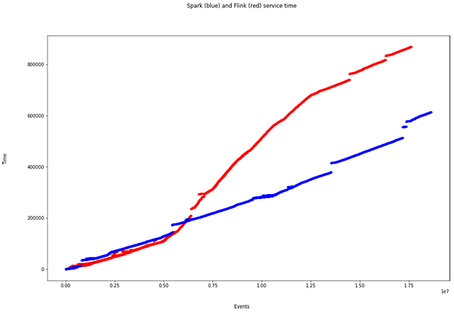
- Spark total time: 614.1s
- Total time Flink: 869.3s
We observe an increase in processing time for Flink. This is due to the way it ingests events:
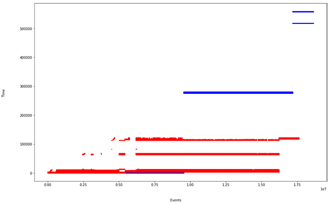
As seen in the last figure, Flink does not use micro-batches and parallelises the event windowing (unlike Spark, it uses overlapping sliding windows). This causes a longer computation time, but shorter ingestion time. It is one of the particularities that we must take into account when defining our streaming Big Data processing architecture.
And what about the calculation?
The Euclidean distance of 10,000 events has the following distribution:
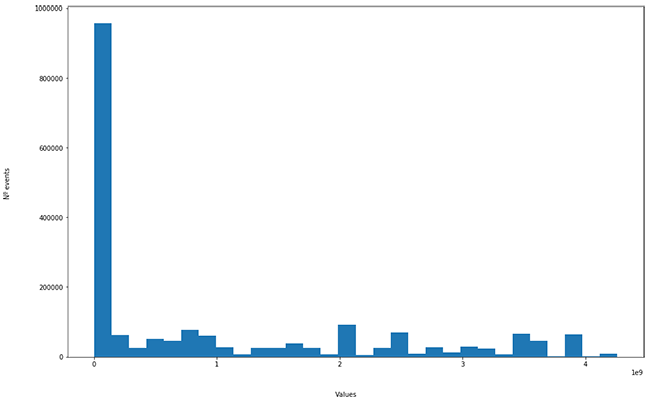
It is assumed that anomalous events are in the “long tail” of the histogram. But does it really make sense? Let’s analyze it.
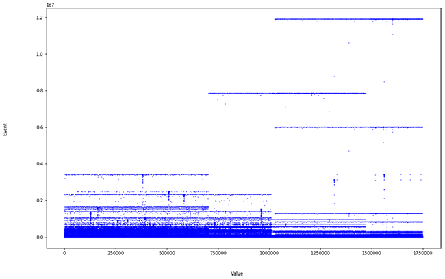
In this case, certain categorical parameters (IP, port) are being considered as numerical for the calculation. We decided to do so to increase the dimensionality and get closer to a real problem. But this is what we get when we show all the real values of the distances:
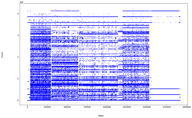
TThat is, noise, since these values (IP, port, source and destination) distort the calculation. However, when we eliminate these fields and process everything again, keeping:
- duration
- in_bytes
- in_packets
- out_bytes
- out_packets
We obtain the following distribution:
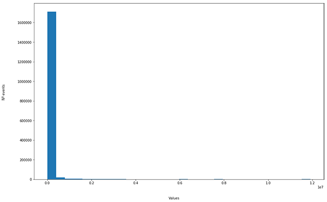
The long tail is no longer so populated and there is some peak at the end. If we show the values of the distance calculation, we can see where the anomalous values are.
Thanks to this simple refinement we facilitate the work of the analyst, offering him/her a powerful tool, saving time and pointing out where to find the problems of a network.
Conclusions
Although an infinity of possibilities and conclusions could be discussed, the most remarkable knowledge obtained throughout this small development is:
- Processing framework. It is not trivial to move from one framework to another, so it is important from the start to decide which framework is going to be used and to know its particularities very well. For example, if we need to process an event instantly and this is critical for the business, we must select a processing engine that meets this requirement.
- Big Picture. For certain features, one engine will stand out over others, but what are you willing to sacrifice to obtain this or that feature?
- Use of resources. Memory management, CPU, disk … It is important to apply stress tests, benchmarks, etc. to the system to know how it will behave as a whole and identify possible weak points and bottlenecks
- Characteristics and context. It is essential to always take into account the specific context and know what characteristics should be introduced into the system. We have used parameters such as ports or IPs in the calculation of distances to try to detect anomalies in a network. These characteristics, in spite of being numerical, do not have a spatial sense among them. However, there are ways to take advantage of this type of data, but we leave it for a future post.
Author: Adrián Portabales-Goberna and Rafael P. Martínez-Álvarez, senior researcher-developer in Intelligent Networked Systems Department (INetS) at Gradiant